Joining data - [Party 1]
In this tutorial, we will walk through a step-by-step process of analyzing sales and nutrition data using the crandas library.
Step 1: Start the engine
First, we import the necessary libraries, including crandas (cd), pandas (pd) and other necessary packages.
import crandas as cd
import pandas as pd
import plotly.express as px
Step 2: Input data
We set the number of rows to read for each dataset and define the table name for the food sales data.
#Set this to limit the amount of data
rows_per_dataset = 1000
food_sales_table_name = 'food_sales'
We then select the relevant columns that we need for our analysis.
# Select relevant columns
relevant_columns = ['Year',
                    'ProductNumber',
                    'ProductName',
                    'EAN_Number',
                    'QuantitySold']
Read the local file and upload it
We read the food sales data from a local CSV file and limit the number of rows to our specified value (1000). After that, we upload the data to the engine using cd.upload_pandas_dataframe()
# Read in the csv to pandas
food_sales_data = pd.read_csv('../../data/sales_nutrition_data/food_sales_data.csv', nrows=rows_per_dataset)

# Upload the pandas dataframe to the engine
food_sales_table = cd.upload_pandas_dataframe(food_sales_data[relevant_columns]).save(name=food_sales_table_name)

# Show metadata for the table (column titles and field types, i=integer, s=string)
>>> print("Table meta-data:", repr(food_sales_table))
    Table meta-data: Name: 4D172B6A3F7412FE967F17D1B5BB98755EAB558B81EB76137849AB20E0F2C6F4
    Size: 1000 rows x 5 columns
    CIndex([Col("Year", "i", 1), Col("ProductNumber", "i", 1), Col("ProductName", "s", 18), Col("EAN_Number", "s", 7), Col("QuantitySold", "i", 1)])
Step 3: Access the Other Party’s Data
Important
Before this step, it is important to execute the script Joining data - [Party 2] and get the table handle to paste in the following code.
Now we can access and connect to the second table containing nutrition data.
# Show that we can access and connect to the second table
nutrition_table_handle = 'NUTRITION_TABLE_HANDLE_GOES_HERE'

# Access the table
nutrition_table = cd.get_table(nutrition_table_handle)
Step 4: Join tables
We perform an inner join on the food sales table and the nutrition table using the EAN code as the key, and account for the fact that they have different column names in each table.
#Join the two datasets using an inner join on EAN code
joined_table = cd.merge(food_sales_table, nutrition_table, how="inner", left_on='EAN_Number', right_on='ean_code')
Step 5: Run the analyses
We compute the average number of products sold and the number of products with zero sales for some simple data quality checks.
avg_sales = joined_table['QuantitySold'].mean()
zero_sales = sum(joined_table['QuantitySold'] == 0)
>>> print('Average number of products sold:', "%.0f" % avg_sales)
    Average number of products sold: 23909
>>> print('Number of products with zero sales:', zero_sales)
    Number of products with zero sales: 2
In the next step, we define a list of labels that represent different nutritional elements in the datasets.
labels_list = ['ENERGY_VALUE_IN_KJ',
                'ENERGY_VALUE_IN_KCAL',
                'SODIUM_IN_MG',
                'SATURATED_FATTY_ACIDS_IN_G',
                'TOTAL_PROTEIN_IN_G',
                'MONO_AND_DISACCHARIDES_IN_G',
                'DIETARY_FIBER_IN_G']
Now, we compute the total nutritional values for each product by multiplying the nutritional element columns by the number of items sold (AantalVerkocht) and store these values in new columns with the suffix _tot.
# For each label (k) listed above, create a "totals" column that multiplies column k times "AantalVerkocht"
merged = joined_table.assign(**{k + "_tot":(joined_table[k] * joined_table['QuantitySold']).astype("int24") for k in labels_list})
After this, we set the year to 2019, define a new list of labels without ENERGY_VALUE_IN_KJ (calories in kilojoules), and create a dictionary coicop to map product numbers to their names. We also create an empty list named table to store the data.
year = 2019

labels_list = ['ENERGY_VALUE_IN_KCAL',
            'SODIUM_IN_MG',
            'SATURATED_FATTY_ACIDS_IN_G',
            'TOTAL_PROTEIN_IN_G',
            'MONO_AND_DISACCHARIDES_IN_G',
            'DIETARY_FIBER_IN_G']

coicop = {1113: 'Bread',
      1117: 'Breakfast cereals',
      1175: 'Chips',
      1183: 'Chocolate',
      1222: 'Soft drinks',
      1184: 'Candy'}

table = []
In this loop, we iterate through the coicop dictionary and labels_list, calculating the total nutritional values for each product and nutritional element in the specified year. We then append this data to the table list and create a DataFrame df with the appropriate column names.
for key,val in coicop.items():
    for label in labels_list:
        sub = []
        sub.append(key)
        sub.append(val)
        sub.append(label)
        sub.append(sum(merged[(merged["ProductNumber"]==key) & (merged["Year"]==year)][label+"_tot"]))
        table.append(sub)

df = pd.DataFrame(table, columns =['ProductNumber', 'ProductName', 'Element', 'Totaal'])
df.head()
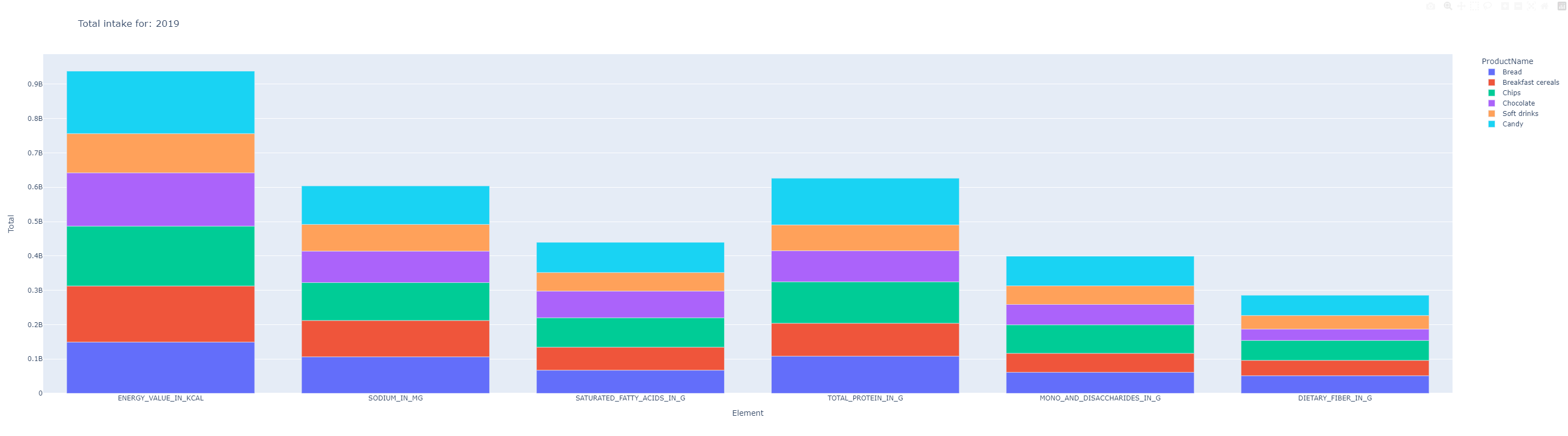
Finally, we create a bar chart using the data from the df DataFrame. The x-axis represents the nutritional elements, the y-axis represents the total nutritional value, and the bars are colored by product names. The chart’s title displays the year of analysis (2019).
fig = px.bar(df, x="Element", y="Totaal", color="ProductName", text_auto=False, title='Total intake for: '+str(year), height=800)

fig.show()