Random forest classification
Introduction
A random forest classifier classifies data into a number of categories by applying a number of decision trees to it. Given a sample, by following the decision tree from the root to the leaves, a probability is derived of that sample belonging to the respective categories. In a random forest, an overall prediction is obtained by averaging the predictions of its respective trees. Random forests are a widely used classifier for tabular data since they can be trained on relatively small amounts of data with little customization.
Crandas provides an implementation of random forests similar to the one offered by sklearn. This user guide shows the steps needed to preprocess training data, fit the model, and apply it.
For more information on random forests generally, see:
Setup
The random forest functionality is available by implementing the appropriate crandas module:
Reading the data
We will demonstrate the use of the random forest classifier by using the well-known "iris" dataset from sklearn. This dataset can be loaded and uploaded into crandas as follows:
from sklearn.datasets import load_iris
import pandas as pd
import crandas as cd
iris = load_iris(as_frame=True, return_X_y=True)
data = cd.upload_pandas_dataframe(iris[0], auto_bounds=True)
labels = cd.upload_pandas_dataframe(pd.DataFrame(iris[1]), auto_bounds=True)
The records of this dataset have four numeric features: sepal length
(cm), sepal width (cm), petal length (cm), petal width
(cm). These features are used to predict the species of iris, encoded
as a value \(0\), \(1\), or \(2\).
In this example, the input columns are fixed point columns, but it is possible to use integer columns as well. It is also possible to use categorical features, encoded as integers (see below).
Creating the model
A random forest model is created by calling
RandomForestClassifier:
>> forest = RandomForestClassifier()
>> print(forest)
RandomForestClassifier(n_estimators=10, max_features=sqrt, max_samples=0.3,
bootstrap=True, max_depth=4), handle=0FCA7F098447E7CD99D91FECB66CD8083...
The random forest classifier has in this case been initialized with the default values for the supported parameters. These parameters can be changed by passing them to the above function, or by setting them for an existing model:
>> forest.n_estimators = 5
>> print(forest)
RandomForestClassifier(max_features=sqrt, max_samples=0.3, bootstrap=True,
n_estimators=5, max_depth=4), handle=A17FC1F6B6AE0B4AC4D16838C939B01...
It is important to note that not just the value of the n_estimators
parameter has changed, but also the handle of the server-side object. In
general, any change to the model, including setting parameters and
fitting (but not using), changes the handle. The handle can be used to
retrieve the random forest model from the server, for example, in
another script:
>> cd.get("A17FC1F6B6AE0B4AC4D16838C939B0163EBD257F7DFEF4267BC6C7F11C1DEE1B")
RandomForestClassifier(max_features=sqrt, max_samples=0.3, bootstrap=True,
n_estimators=5, max_depth=4), handle=A17FC1F6B6AE0B4AC4D16838C939B01...
Fitting the model
The model can now be fit to the training set that we created earlier.
Fitting the model is done by calling
RandomForestClassifier.fit():
The class labels need to be encoded as boolean values or as integers
\(0,\dots,C-1\), where \(C\) is the number of classes. For integer values, the
number of classes needs to be specified as an argument to the fit
function (unless it can be derived from the column metadata; see
RandomForestClassifier.fit() for
details).
By default, all features are assumed to be ordinal (containing numbers,
using the decision criterion \(val \leq T\)). A feature can be specified as
being categorical (containing categories \(0, .\dots, C-1\), using the
decision criterion \(val = T\)) using the categorical_features argument
to RandomForestClassifier.fit().
As long as the number of different categories is relatively small, fitting a
categorical feature can be much faster than fitting an ordinal feature.
For a categorical feature with values \(0,\dots,C-1\), the number of
categories needs to be specified in its ctype, e.g., by passing
data.astype({"feature": "int[min=0,max=2]"})) as argument to the fit
function.
Detailed information about the fitted model can be retrieved by using
the .attributes attribute of the fitted model, or by inspecting
specific attributes (see RandomForestClassifier):
>> print(forest.feature_names_in_)
['sepal length (cm)', 'sepal width (cm)', 'petal length (cm)', 'petal width (cm)']
>> print(forest.n_classes_)
3
Predicting
Once the model has been fitted, the function
RandomForestClassifier.fit() can be used
to apply it to a dataset to make predictions. The dataset needs to have
the same columns and column names as the original data that was used to
fit the model; use .rename() to
update column names if needed.
>>> forest.predict(data).open()
    target
0         0
1         0
2         0
3         0
4         0
..      ...
145       2
146       2
147       2
148       2
149       2

[150 rows x 1 columns]
It can be verified that the model has correctly predicted the type of iris in most cases:
Instead of getting the output classes, it is also possible to get the respective class probabilities:
>> forest.predict_proba(data).open()
            0         1         2
0    1.000000  0.000000  0.000000
1    0.838095  0.152380  0.009523
2    0.838095  0.152380  0.009523
3    0.838095  0.152380  0.009523
4    1.000000  0.000000  0.000000
..        ...       ...       ...
145  0.000000  0.018182  0.981816
146  0.000000  0.018182  0.981816
147  0.000000  0.018182  0.981816
148  0.000000  0.018182  0.981816
149  0.000000  0.018182  0.981816

[150 rows x 3 columns]
Inspecting the trained model
Detailed information about the fitted model can be obtained by opening
it, using the open() method. This provides the full data
representing the model. This data can also be used to upload a copy of
the model using from_opened(),
e.g., the following creates a copy of the model:
import crandas.crlearn.ensemble
>>> crandas.crlearn.ensemble.RandomForestClassifier.from_opened(forest.open())
RandomForestClassifier(max_features=sqrt, max_samples=0.3, bootstrap=True,
n_estimators=5, max_depth=4), handle=0C7CD71C566BED10C137B04373ACA1...
A more user-friendly representation can be obtained by converting the
trees of the model to a pydot graph representation. This graph
representation can be visualized, e.g., as follows in Jupyter:
opened = forest.open_to_graphs()
opened[0].write_png("out.png")
from IPython.display import Image
Image("out.png")
This displays the first fitted decision tree, which can for example be
as follows (here, for simplicity a tree is shown that has been fitted
with the parameter max_depth=2):
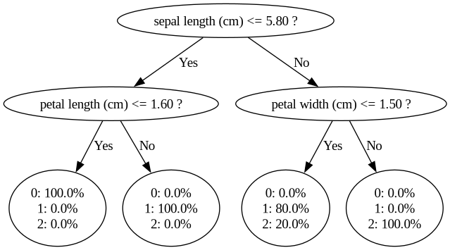
In this particular decision tree, first, it is checked if the sepal
length is at most 5.8. If so, it is checked if the petal length is at
most 1.6. If so, the flower is classified with 100% probability into
class 0. Similarly, if the sepal length is greater than 5.8 and the
petal width is at most 1.5, then the flower is classified with 80%
probability into class 1 and with 20% probability into class 2. The
overall classification corresponds to the highest average probability
over the fitted trees.